| Notes on
Bos, HJ ( nd) 'Differentials, Higher-Order
Differentials and the Derivative in the
Leibnizian Calculus' ,
www.tau.ac.il/~corry/teaching/toldot/download/Bos1974.pdf Dave Harris The story so far, as far as I understand it. There was a problem in calculating changes in direction or slopes of lines in graphs. The problems seemed to lie in the observation that the line was a continuous variable, an infinite series of points. This meant that strictly speaking, areas and the like could not be calculated with precision, because there was always an area extending beyond the artificial point to which we had given a number, and units were fundamentally arbitrary. That was OK if we stuck to the (rather mysterious) geometric dimensions (the normal 3?) . However, a further reservation meant that this would be confined only to solid objects and their geometries—beyond that, we had no agreed dimensions and therefore no agreed quantities.This prevented any further abstraction, so that points on the graph for Descartes remained as single concrete calculations, as it were, not more abstract functions but concrete relations between discrete variables. Apparently, Descartes had attempted to tackle this by providing a series of algebraic equations to explain the slope of a curve in terms of variable quantities of X and Y. This included working with ratios between lines (line segments) which would be precise. If we let algebraic terms stand for those line segments, we can multiply the terms. We do not need to use real numbers. We can substitute real numbers for solutions, but that involves an arbitrary operation of choosing units again. Leibniz is going to generalize to take ratios even further away from real numbers and geometric dimensions, and make them into functions: he was one of those who coined the term along with Bernouille and Euler (incidentally, they had to agree on terms -- another was the 'integral' which Bernouille preferred to Leibniz's term 'sum'). Originally, Euler's functions related to single variables, later to many, another move from geometric space. He is going to establish a ratio between changes in x and changes in y, dx and dy. Changes are to be expressed in an abstract way not arithmetic, as differentials. He still has problems though with the notion of the infinitely small, and will lead to a replacement for Leibniz's system -- a further abstraction from the specific calculations of differentials based in infinitessimals -- the derivative. It seems that this dilemma shows a move from geometry to analysis is how Bos describes it, or a move towards the concept of a mathematical function, where one variable maps on to another. Mathematicians became more interested in these generally, and stopped worrying about real world equivalents (scholasticism -- but what machinic possibles unfolded!). Leibniz began his inquiries with the geometry of graphs and the function emerged. Terms become fully abstract symbols. Leibniz had already investigated the issue of differentials to explain sequences—the differences between one number and another, one solution and another. Again there are regular mathematical formulae to explain how these differentials can add up, and you don't have to be much of a philosopher to realise that infinitely small differences lie at one end and infinitely large sums of these differences at the other. The work was done originally on number sequences so Leibniz had to extrapolate to changes in coordinates on graphs -- he saw that differentials could be used to explain the use of tangents, and sums the 'quadrature' (area under the curve) .This helps us explain the slope of a tangent as changes on the X and Y axes of a graph without actually putting any values or numbers (real numbers to be precise) on them. What about curves representing a relation between the Y axis and the X axis? Common sense suggests that we can pretend these curves are straight lines, by drawing a tangent to the curve as a hypotenuse of a triangle (the other two sides being distances on X and Y). A simple tangent on a sharp curve (NB tangents always connect two points on a curve at infinitely small distances from each other) will obviously include bits outside the curve, however. To try and pin down that area we can draw another tangent that turns that area into a triangle, then subtract it from the first total. Again there will be surpluses, so yet another triangle can manage those—and so on to infinity. Apparently, Leibniz said that what we were doing is drawing an infinitely sided polygon from an infinite number of tangents touching the curve, together with the familiar three sided square, so to speak, provide by lines on X and Y axes connecting to the tangent. We then have to remember we are not assigning real values to the areas of the triangles, because the hypotenuses are infinite, but comparing their differences as we move round the curve: we have to do this with continual variables. It is the best we can do to make the infinite finite -- we can at least generate finite sequences (based on the earlier application to numbers?). So the variable becomes understood as an infinite sequence of differentials, a series or progression (sometimes Leibniz uses terms that imply progression or growth). As we approximate more and more closely the shape of the curve, the differences (residues) get smaller and smaller. So we now have two key operations. Calculating the differences between the triangles that we draw, the differentials, which are infinitely small, represented as a triangle or d. Then we have to add these differences up to infinity, the infinitely large, to get the area of the quadrature, using sigma, represented as the elongated S. The change in terminology represents a change from concrete operations of calculating difference and adding them, to abstract operators which can range to infinity in both directions. As hinted above, Leibniz's original term of summing was replaced after conversation with these friends to that of integration. With this abstract operation, we also move to the idea of a function, applicable to any range of real values, and applying equally well in reverse, so there is no longer a difference between dependent and independent variables. In practice, the extremes of the infinite were largely ignored, but an additional problem arose in calculating 'higher order' (secondary) differentials ('variables ranging over an ordered sequence'), (17) Now a really clever bit. Ratios again. Draw a tangent and extend it down to the x axis. Make it a triangle with the 'subtangent' (the length on the x axis from the point at which the tangent crosses the x axis to the point at which the y coordinate drops from the tangent to the x axis. The 3 sides of this triangle are known as alpha (subtangent) Greek y (height from x axis to tangent) and Greek r, length of tangent ( see diag below, p. 18). The ratio between these 3 will be the same as the ratio of the sides of the differential triangle. I think this only holds if we want to extend a regular curve to infinity. In effect, the original triangle gets infinitely repeated.   This is
obviously a version of the triangle that
Deleuze (The Fold) and Delanda get
so keen on:
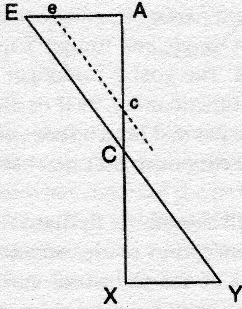 Here, the ratio stays the same as we reduce the dimensions of the triangle from E to e and C to c etc. When we locate the line ec exactly on A, the actual values of the lengths of the lines are 0 -- but the ratio remains, fully free of the real world. I am not sure if the values really are at 0, though, not at the infinitely small -- perhaps it is the same thing for all intents and purposes? We can see the same development in Bos's diagram of course --just project the triangle further and further to the right, into the infinitely small. Incidentally, all equations could be said to remain as a relation when the actual values are zero? Maybe this is the point -- the triumph of the relation. So. we began with a measurement problem solved by turning to differentials and ratios. We saw that sequences of differentials can extend to the infinite, as infinitessimals. And this is where we have ended -- 'pure' ratio. Back to the Le9obniz version, I suppose this does help us see the shape of curves especially since it is about the relation between changes. and their analogous(?) relation to actual lengths. Another thought strikes me -- if the ratios change will this help us explain changes in the slopes of the curve? If Y increases, will this not affect the slope? I think this is what is at stake in needing to develop the higher order differentials and sums. The values of dx and dy can and often do change, and, guess what, we can assess that as a differential too -- ddx and ddy. And do the same to get dddx etc Same with sums. Again, differentials will tend to the infinitely small, and sums to the infintely large. Then we get on to the relations between differentials and sums [dear God, but apparently we must!]. It is easy to see that the sum of all the differentials of y is y itself -- $dy=y. But it is also true that d$y =y ( hard to put this in normal English. If I have glossed Bos correctly, (19) it means that the differential/differences between the terms in the sum of all the values of y is y itself. Bos says we can see this better if we think of the differences between the items in the sum as prdued by infinitely small quadratures in the first place -- but I still don't really get it. I think the argument is that as we continue to add infinitely small quadratures we get close to the actual variable, and when we get to adding quadratures of 0 size, we are completing this process. I will just have to accept for now that d and $ are reciprocals of each other]. Horrible but perfectly logical complications ensue,such as that the differential and the integral themselves enjoy a 'pure' relation, as inverses of of each other. I am also glimpsing a 'practical' implication, if we accept that the practical problem was measuring the area under complex curves. It will be the sum of all the areas of quadratures produced by adding tangents to the slope of the curve. And (maybe) we can see that sum as the reciprocal of the sum of all the differences between points on the curve? Back to the abstract maths. There is now an operation called integration which 'assigns to an infintely small variable its integral', accepting by definition that 'the differential of the integral equals its original quantity' (20) (as in $dy=y above?). This is where Leibniz and Bernouille agreed to use the latter's term integral rather than sum ( 21)This is a further abstraction from the process of adding the incremental quadratures. We can reinterpret this adding to mean not just that in any particular case, an overall quadrature is made up of the sum of all the little quadratures, but that the overall area of the quadrature can be rendered as the differential of the little quadratures that make it up. Remember that calculating the area of the overall quadrature is our practical aim. I don't know if we are ever going to be able to substitute real values for the differentials? We can quantify relations though. Across a finite range no doubt we could actually measure changes in x and y etc? . With unconfined ranges it is difficult because we would have to keep adding areas to the infinitely large. We have avoided this again (made it less likely is how Bos puts it) by thinking of quantified relations not actual values We can manipulate these quantities in relations. We can preserve the original dimensions to which they refer ( so on a conventional graph we are measuring differences in lengths of a line etc). Then some more stuff which I have to take on trust. We assume the polygons ( little quadratures) are regular and this somehow leads us to assume that the measures of relations are also regular - -kind of nested is how I see it, so differentials ( and sums) stretch away to infinity compared to actual numbers, and higher oirded differentials (and sums) do the same for the differentials. I think this is an assumption that helps us manage concepts of the infinte using the same principles An arcane dispute reported on 23 led to Leibniz proving that higher differentials were infinitely small compared to differentials but were still quantities. Then -- 'first order differentials involve a fundamental indeterminacy' (24) because the formal definition of a differential as ,say a line segment of a certain length applies to segments of many lengths ( so the definition is too pure as it were) , and there are also segments of other lines, related to x which would also agree. This was not notiiced originally, and makes no difference for practical calculations in normal geometry ( who cares exactly how small a segment is at the infinitely small level, and who cares is there are other possible mathematical lines). A bigger problem arises though. What sort of polygon do we draw to represent the quadratures? Again I am forced to gloss, but the issue seems to be that the ratios will vary according to how we draw the polygon -- equal x sides? Equal y sides? Equal sides? ( I must confess I don't see how the x or y sides could be equal, but there -- ah, these are projected sides. But if we project we are surely making the x sides artificially equal and I can see how this will screw up the ratios, so why do it? Perhaps we have to if we cannot directly measure? ). We also need to make assumptions about the changes in the dimensions of the differential triangle above when we get to infinite levels ( thought so). We have to assume one or all three of the sides remains constant. These can only be reasonable suppositions or 'choices' ,and we might wish instead to suppose rates of change ( eg by working out the combinations of varying each side in turn to give 18 possibilities, apparently, and assuming uniform change) . Guess what -- there are really infinite choices and thus an infinite range for the changes in the sides. We have to pin it down somehow or the differentials (and sums) will be indeterminate again, capable of occupying any position on the range, from 0 (no alteration in change) upwards. We can only deal with this if we consider the area of each additional little quadrature (which will vary if the sides of the triangle vary) ,and the overall quadrature as the sum of them. It will be dead handy if one of the sides only varies. At the end of the day, we just have to assume there is some regularity in the little quadratures and just exclude 'anomalous progressions'. Again this is OK for practical purposes if the anomalies are infinitely small. Apparently we will still have problems with 'singularities', (the points at which the curve changes direction?). In effect, by assuming constant change in one variable, we are suggesting that this can be an independent variable ( a common procedure in stats etc) . Again this is OK with most actual calculations, but there are still problems in theory (one of them turns on whether 0 is a point on a journey to infinity -- 28). Another development is required to fully deal with indeterminacy without making assumptions about rates of change in variables. We have to calculate the slope of curves by calculating differential equations, the rates of change of the variables. Differential equations proceed by following certain rules ( god knows where these come from -- well from Leibniz it seems) p.29, which hold whatever concrete values apply to the progression of the variables ( although it is still common in practice to hold one variable constant etc) It cut out the need for long calculations with actual curves etc. I am lost again, but what we have to do is take the (conventional, Cartesian? ) formula for a curve (the example is ay=x sqd which gives you a parabola, where a is any number?) and apply the operator d to both sides ( and how do we derive that exactly? I am still stick with a need to give a concrete value to d!). We can get closer and closer to the shape by repeatedly differentiating as in higher-order differentiations, which get closer and closer to infinity etc. We still need to specify if the differential equation applies to x or y, though, which still involves a choice of holding one constant, at least at one stage. It follows we can predict the shape of a curve if we enter values in the differential equations. Oh good -- there are formulas for calculating derivatives after all ( but I don't understand them), varying according to whether x or y is held constant -- eg y(x=sq rt ay) apparently gives you the derivatives of x. Remember a=a line segment or quantity of length. Derivative is the calculation of the rate of change. I need to keep reminding myself. I also need a break -- off to paint windowcills |